Welcome to MakerHome


We've completed our yearlong print-a-day project!
All new material is now at Hacktastic: www.mathgrrl.com


Saturday, August 16, 2014

Day 355 - Saturday guest: Fred Hohman and knot fibrations, part 1

One thing about living in New York City is that you get a lot of guests. Lots of people come to the city and hotels are too expensive even to consider! We've had seven different people visit us since we moved here just a couple of months ago. Blog-wise it's the same story: now that the print-a-day year is wrapping up we have a lot of guests. Welcome all!

Today's guest poster is Fred Hohman (fredhohman on Thingiverse), an undergraduate mathematics student at the University of Georgia, student of David Gay as well as my good friend Jason Cantarella. Fred is the designer of the beautiful "trefoil trumpet" we printed on Day 311, and in the next two posts he'll be walking us through the math and the Mathematica of a sort of "3D puzzle" based on this trefoil. 

Hello MakerHome and MakerHome readers!

I am Fred Hohman, a rising senior Mathematics and Physics student at the University of Georgia. I have been working under Dr. David Gay in the Department of Mathematics at the University of Georgia since the beginning of the year, and I will be continuing my work until my graduation in May 2015.

Earlier in the summer I had the wonderful opportunity to meet Dr. Laura Taalman (mathgrrl) after her talk at MoMath on “Making Mathematics Real: Knot Theory, Experimental Mathematics, and 3D Printing.“ After chatting about math and 3D printing she asked me say some words about my undergraduate research at UGA. You may have seen already Dr. Taalman’s earlier post “Day 311 — Trumpet Trefoil,” in which she introduced my trefoil knot. If you have ever seen a standard trefoil knot you’ll notice that the trefoil that was depicted is a bit different.

The goal of this project is to create a 3D puzzle of the trefoil knot and its fibrations via 3D printing.

Let’s start with some theory.

Theory and Stereographic Projection.
Consider the following function from C^2 to C (we can think of this as a function from R^4 to R^2 - see the Wikipedia entries for real n-space and complex n-space for more information): this function sends a coordinate pair (u, v), where u and v are complex numbers, to the quantity (u+i*v)^2-(u-i*v)^3, where i = sqrt(-1). This particular function’s zero-set, a set of points {(u,v), …} such that (u+i*v)^2=(u-i*v)^3, generates a trefoil knot through infinity. By considering inverse images of certain subsets of C we will generate a trefoil knot given our function’s zero-set; however, this inverse image is a subset of C^2. To obtain our knot and understand its subsets better, we need a method to realize our object in R^3.

As a preliminary example, consider a sphere in R^3 sitting on a plane (think of a ball sitting on a table). From the top of the sphere (think North Pole), draw a line segment downward through the sphere and ending at the table. Notice that this line segment intersects both the sphere and table once. We can do this same line drawing method over and over to obtain a one-to-one correlation from the sphere to the plane, i.e., every point (well, minus the exact top of the sphere!) on the sphere can be mapped to the plane. This is called stereographic projection, and Henry Segerman (henryseg on Thingiverse) has created a fantastic 3D printed model illustrating this method:


If we have a point light source (smartphone camera flash) and place it at the top of this model, light rays will act as the line segments in the above example. If held at the correct height, we should see the Cartesian grid on the table. I always keep this model in my backpack to demonstrate to people stereographic projection—I recommend printing it out!

So stereographic projection is a function from the unit sphere in R^3 onto R^2, but recall that our function is defined in R^4. For us to embed our object in R^3, we use a generalized version of stereographic projection to go from the unit sphere in R^4 to R^3. With this tool, we can compose the inverse stereographic projection function with our function defined above. So our new function now goes from R^3 -> C.

If we take inverse images of subsets of C, we now have a function that goes from C -> C^2 = R^4 -> R^3, i.e., our single, final function takes in certain subsets of C and outputs subsets of R^3—exactly what we want!

Mathematica, Plotting, and Resolution.
To generate 3D computer models of the trefoil knots, I chose to use Mathematica. RegionPlot3D, a built-in Mathematica function, plots regions in 3D space using inequalities. In order to use RegionPlot3D, the user must specify the domain of values to plot over in the x, y, and z directions, as well as a mathematical inequality. As an example we can generate a sphere of radius 1 by the following code:


Mathematica will plot all points (x, y, z) such that each point falls within the considered domain and obeys the given inequalities—but we can take this further. We can use multiple inequalities using boolean operators such as AND and OR. As an example, let’s consider the same sphere defined above, but restrict the region so that only points above the plane z=0 are plotted.


Of course we could restrict the z range so that z goes from (0, 1), but it is nice to be able to manipulate a model without changing the overall plotted region. When models become more complicated this method allows us to control individual components without altering other pieces.

Before we start creating trefoil knots, there is one last Mathematica option that needs to be discussed: PlotPoints. Notice how choppy and non-circular the bottom of our hemisphere looks in the image above—PlotPoints will fix this. The PlotPoints function can be thought of as the resolution of a 3D model. A higher PlotPoints value tells Mathematica to use more points to represent the plotted region. However, as we increase PlotPoints, we also increase computation time. Say we used a PlotPoints of 50 and the model was under-represented. We could double our resolution and set PlotPoints to 100, but remember we are in 3D space, so by doubling the number of points in all directions (x, y, and z) we increase our computation by 2*2*2*=8. In other words, doubling a model’s resolution increases computation time by a factor of 8. So let’s plot that same hemisphere with a PlotPoints of 100 and see what the bottom looks like.


Much better! Now that we have an understanding of RegionPlot3D and PlotPoints, it’s time to create some trefoil knots.

The main Mathematica function I wrote, inTinftube, defines the trefoil knot (the composition of our trefoil knot function with inverse stereographic projection explained above) by inputting points (x, y, z) and “knot thickness” and returning a single number. Inside the function it tests points using inequalities such that if the outputted number is less than 0, Mathematica includes the point in the plot, and if the number is greater than 0, Mathematica does not include the point in the plot. We also need to define a boundary condition, otherwise our model would stretch to infinity! So we can include more inequalities that points must satisfy such that our boundary is a cylinder of radius 3, height 6, and is centered at the origin. With these parameters selected, the results below depict our “standard” trefoil knot. This knot is the inverse image of a small disk around 0 in C to give the knot thickness—a visual description of this will be shown in the next section.


Thingiverse link: http://www.thingiverse.com/thing:243260

Open Book Decomposition, Fibrations, and Pages.
Now that we have our “standard/reference trefoil knot,” it is time to start adding fibrations. To do this, unravel the above trefoil so that it is a straight strand. Consider that cord the spine of a book. Now add in one page to the book; the page will connect to the spine along one edge. Now twist the cord back into the trefoil knot configuration—what does the page, i.e., knot fibration, look like? This idea is called an Open Book Decomposition.

We can visualize this by adding extra regions to the model in C before we apply our single function. To do this, I wrote another Mathematica function, inTinfpage, that takes in points and outputs a number; however, this time the function also requires an angle. This angle will define a ray in the plane starting at the origin that is rotated an angle in the mathematically positive direction. As before, we can have Mathematica plot points if the outputted number is below zero, but we want a page of some physical thickness (in order to 3D print). For most of my successful prints I have been using a page thickness of pi/6. So we can now include another “ray-function” and input an angle that is pi/6 larger than before and have Mathematica plot things that are greater than 0. We have now included another region in the plane. This process is much easier to see in the image below.


The circle is the radius of the trefoil knot, and the region in the first quadrant is our fiber with thickness. That’s the new region we want to include when using stereographic projection. Remember the picture above is the subset of C that we are taking inverse images of. We can now apply our same code to generate the following model.


Why stop at one extra region? We can add as many as we would like, and at pi/6 thickness, we should be able to fit 12 extra regions in our trefoil knot (since pi/6*12=2*pi). Some other examples are below, with the region in C shown on the left, and its inverse image (after applying stereographic projection) shown on the right.


We can now start to see the consequences of projecting our 4D function into R^3, which is why our knots are visually unlike typical trefoil knots.

In the next post we'll 3D print the models we have created...

Friday, August 15, 2014

Day 354 - Forty-one Pentagonal Icositetrahedra

Today (August 15) I had the great pleasure and honor of attending the final convocation for the 2014 NYU GSTEM program. At this event, 41 young women who are rising high school seniors presented the work they did this summer interning at various science, technology, engineering, and mathematics departments. The presentations were incredible and if I hadn't known they were high school students I would have thought they were just finishing college and on their way to graduate school. Today the future looked very, very bright. Like, genius bright. We made them each a Pentagonal Icositetrahedron (see Day 197).


Thingiverse link: http://www.thingiverse.com/make:90906

Settings: Printed at 50% scale on a MakerBot Replicator 2 with .2mm layer height and raft but no support (hooray!).  Print time was about 21 minutes a piece and they printed eight-up without problems.

Here are some of the are future geniuses looking at the 3D-objects we brought to the convocation:


Thursday, August 14, 2014

Day 353 - Customizable hinge/snap Tetrahedron net

Today we modified Day 344's Cube net design to make a Tetrahedron net:


Here it is mostly folded up. This net is so small that it only folds well in one direction; in the other direction the edges of the faces keep the hinges from swinging open enough for the model to close all the way. The cube net, and all other larger nets, fold well both ways.


Thingiverse link: http://www.thingiverse.com/thing:440001

Settings: We optimized this design for printing on a Replicator 2 with .3mm layer height and no raft, no supports. If your printer is different then you may need different clearances in your model. You can use the Thingiverse link to open the model in Customizer and set your own side length, border width, hinge clearance, and snap tolerance.

Technical notes, platform/raft edition: These hinge/snap net models print best without a raft. You can print them with a raft, but it will take 50% as long and then another 25% longer for you to peel off the raft bits. (Note that although you can print these with rafts if for some reason you want/have to, you cannot print these models with supports or the hinges will not work correctly.) If you're printing on an acrylic build plate with PLA, like the standard plate that comes with the MakerBot Replicator 2, then you have an excellent build surface for printing without a raft. If you're printing with a glass platform on the Replicator, or with some other printers, then you may not be able to print without a raft. For me at least, PLA never sticks to the glass, and I need glass+tape+raft to make prints work on the glass build plate (see Day 214). In any case, make sure your build platform is very level before you try printing a large hinge/net model, or the outer pieces will be deformed and hinges and snaps may fail.

Technical notes, OpenSCAD edition: Using the same hingesnappoly_maker, and attach modules as on Day 344, we assembled the tetrahedron as follows:

// center triangle
union(){
poly_maker(sides=3);
attach(type=2,side=1,sides=3);
attach(type=2,side=2,sides=3);
attach(type=1,side=3,sides=3);
}

// next triangle
translate([ (length/tan(180/3)+jump)*cos(180/3),
(length/tan(180/3)+jump)*sin(180/3),
0]) 
rotate(180/3,[0,0,1])
union(){
poly_maker(sides=3);
attach(type=2,side=2,sides=3);
attach(type=1,side=3,sides=3);
}

// next next triangle
translate([ 0,
2*(length/tan(180/3)+jump)*sin(180/3),
0]) 
rotate(2*180/3,[0,0,1])
union(){
poly_maker(sides=3);
attach(type=1,side=2,sides=3);
attach(type=2,side=3,sides=3);
}

// next next next triangle
translate([ (length/tan(180/3)+jump)*cos(180/3),
3*(length/tan(180/3)+jump)*sin(180/3),
0]) 
rotate(3*180/3,[0,0,1])
union(){
poly_maker(sides=3);
attach(type=2,side=1,sides=3);
attach(type=2,side=2,sides=3);
}

Wednesday, August 13, 2014

Day 352 - Center of mass demonstration

Today we printed designbynumbers' Center of mass manipulatives for calculus classes from Thingiverse. It worked very well and balanced wonderfully!


Thingiverse link: http://www.thingiverse.com/make:90962

Settings: Printed on a MakerBot Replicator 2 with .2mm layer height. We changed the infill to "linear" instead of "hexagonal" because the hexagon-filled one seemed not to balance quite right. With linear infill the balance was spot-on.

Tuesday, August 12, 2014

Day 351 - Impossible Menger Burr

After richgain's excellent guest posts walking us through Burr Tools on Day 348 and Day 349, we couldn't resist giving it a try. As I think we've established, I love Menger sponges and I'm kind of a jerk. So I made a burr puzzle that can never be assembled.


Thingiverse link: http://www.thingiverse.com/thing:439478

Settings: The red menger cube was printed on a Replicator 2 at .3mm layer height in 10 minutes, without raft or support, on an acrylic platform. The white cross was printed on another Replicator 2 (don't judge, they had a warehouse sale for the last remaining Rep2's and... well...) at .3mm layer height in 8 minutes, with raft and support on a glass platform with tape.

Technical notes, Burr Tools flavor: I have to give serious thanks and appreciation to the author of Burr Tools, Andreas Roever. Burr Tools has a lot of features that I haven't even attempted yet, including triangle and sphere grids and a whole lot more. And it's free. In addition it solves the puzzles you construct. And it's smart about it; for example, the menger+cross puzzle I made has a solution if you can get the cross into the cube. So it has an "assembly". But it doesn't have a "solution" because you can't actually perform the assembly. This is reported correctly by Burr Tools in the left column of the picture below. Very impressive and useful!


Thanks also go out to Derek Bosch, himself a creator of amazing and intricate puzzles, who wrote the code for the OSX port and also sent me a direct link to the most updated version of Burr Tools so I could run it on my Mac. Here's that link: http://sourceforge.net/projects/burrtools/files/latest/download .

Monday, August 11, 2014

Day 350 - Triple Bubbles

When three bubbles intersect, they do so in a very specific way. Here's what it looks like:


Using the OpenSCAD code for this design included at the bottom of this post you can make your own bubble model with any three bubbles you like. The code will automatically position the bubbles correctly and create the correct surface components that intersect in the center of the model. Or, to print exactly the model above, use the Thingiverse link.

Thingiverse link: http://www.thingiverse.com/thing:438777

Settings: This is very large model that took up most of the build plate of a MakerBot Replicator 2 and printed at .2mm layer height with raft but no supports. It took many hours but we forgot to make a note of exactly how many! So, just, a lot.

Technical notes, math flavor: This model was requested by MoMath to use as a cake centerpiece for mathematician Jean Taylor's 70th birthday party. Jean Taylor famously proved that Plateau's Laws hold for minimal surfaces in her paper The structure of singularities in soap-bubble-like and soap-film-like minimal surfaces.  According to Plateau's Laws, three bubbles will meet at 120-degree angles - just as in the center of the model shown above. However, the three surface components that meet at the 120-degree angle are not flat; they are curved. Each of the three components is a part of a larger sphere whose center lies outside of the bubbles. The three centers are shown by the points F, G, and H in the diagram below, taken from S.M. Blinder's Wolfram Demonstration Three Coalescing Soap Bubbles.


We used S.M. Blinder's Demonstration code to get the mathematical descriptions of the points F, G, and H given the radii of the three intersecting bubbles.

Technical notes, failure flavor: This model left a particularly large trail of fails; below is one that was designed with a much coarser mesh. The coarseness of the mesh left some gaps at the joins between the surfaces, which cased the model to separate. In addition we tried to print the entire top without supports, which caused the problem on the smallest sphere that led us to cancel the print. Most models can be made rather coarsely and still look fine, but this particular model needed a mesh with a very high degree of accuracy to even print correctly.


Technical notes, resolution flavor: To get a fine enough resolution for successful printing, we had to use a lot of triangles in our mesh. The hard part was getting the interior surface segments to contain enough triangles, since they came from much larger spheres. The key to doing this was using very small numbers for the fragment angle and fragment size of the spheres: 

fragA = 2; // fragment angle
fragS = 2; // fragment size

Here's what the mesh looks like in OpenSCAD:


Because of the high resolution needed to make components of this model intersect successfully, I am not putting its OpenSCAD code on the Thingiverse Customizer. I think it would hang or crash to try to run this online. If you're interested in making different bubble configurations then download OpenSCAD and run the code at the bottom of this post, changing the bubble radii as desired. 

Technical notes, OpenSCAD flavor: This was one of the most difficult things that I've made in OpenSCAD. When MoMath asked me if I could design this triple-bubble model, my first reaction was that I had absolutely no idea how to do that, so probably not. But a bit of poking around on the web led me to the excellent triple-bubble Wolfram Demonstration, and they had already done all of the math! I tried to export the Wolfram object using Mathematica, but it was not the right kind of graphics object to allow an STL export. This meant that it had to be reconstructed from the ground up in OpenSCAD. Alas, this in turn meant that I really needed to understand all the mathematics in the code, and also translate the code from Mathematica syntax to OpenSCAD syntax. All this together with the need for high-resolution accuracy meant that this project took many days to put together and get working correctly. 

The OpenSCAD code starts with any three radii for the bubbles and then positions the spheres correctly, computes the center coordinates of the larger spheres that determine the intersecting surface components, and then uses unions, differences, and intersections to output the correct sections of the three bubbles and thee surface components. Because it would be difficult to see the inside intersections if the bubbles were printed as full spheres, the final step is to cut off the top and bottom of the model. This also makes the model very easy to print. 

// mathgrrl triple bubble

////////////////////////////////////////////////////////////////
// bubble radii 

a = 60;
b = 56;
c = 44;

////////////////////////////////////////////////////////////////
// resolution parameters

th = .9; // thickness
fragA = 2; // fragment angle
fragS = 2; // fragment size

////////////////////////////////////////////////////////////////
// scale and render

intersection(){
build_bubbles();
cube([250,200,70],center=true);
}

////////////////////////////////////////////////////////////////
// translation coordinates
// based on code from Wolfram Mathematica Demonstrations Project
// http://demonstrations.wolfram.com/ThreeCoalescingSoapBubbles/

ab = sqrt(a*a+b*b-a*b);
ac = sqrt(a*a+c*c-a*c);
bc = sqrt(b*b+c*c-b*c);

f = 1/(1/b-1/a);
g = 1/(1/c-1/a);
h = 1/(1/c-1/b);

// translation coords for sphere b
xb = ab;

// translation coords for sphere c
xc = (pow(ab,2)+pow(ac,2)-pow(bc,2))/(2*ab);
yc = (-1/(2*ab))*
     sqrt( -pow(ab,4)
-(pow(ac,2)-pow(bc,2))*(pow(ac,2)-pow(bc,2))
+2*pow(ab,2)*(pow(ac,2)+pow(bc,2)));

// translation coords for interface sphere f
bf = sqrt(pow(b,2)+pow(f,2)-b*f);
xf = ab+bf;
yf = 0;

// translation coords for interface sphere g
cg = sqrt(pow(c,2)+pow(g,2)-c*g);
xg = (ac*xc+cg*xc)/ac;
yg = (ac*yc+cg*yc)/ac;

// translation coords for interface sphere h
ch = sqrt(pow(c,2)+pow(h,2)-c*h);
xh = (-ch*xb+bc*xc+ch*xc)/bc;
yh = (bc*yc+ch*yc)/bc;

////////////////////////////////////////////////////////////////
// module for sphere parts and dividers

module build_bubbles(){
//first bubble shell fragment
difference(){
sphere_a(open=1,fudge=0); // start with first bubble shell
intersection(){ // take away the part of the shell
sphere_a(open=1,fudge=0); // that intersects the
union(){ // second and third bubbles
sphere_b(open=0,fudge=-th);
sphere_c(open=0,fudge=-th);
}
}
}
//second bubble shell fragment
difference(){
sphere_b(open=1,fudge=0); // start with second bubble shell
intersection(){ // take away the part of the shell
sphere_b(open=1,fudge=0); // that intersects the
union(){ // first and third bubbles
sphere_a(open=0,fudge=-th);
sphere_c(open=0,fudge=-th);
}
}
}
//third bubble shell fragment
difference(){
sphere_c(open=1,fudge=0); // start with third bubble shell
intersection(){ // take away the part of the shell
sphere_c(open=1,fudge=0); // that intersects the
union(){ // first and second bubbles
sphere_a(open=0,fudge=-th);
sphere_b(open=0,fudge=-th);
}
}
}
//interface between first and second
intersection(){
sphere_ab(open=1,fudge=0); // take only the arc of the circle
difference(){
sphere_a(open=0,fudge=0.1); // that intersects the first bubble
sphere_ac(open=0,fudge=-th); // but not the other interface
}
}
//interface between first and third
intersection(){
sphere_ac(open=1,fudge=0); // take only the arc of the circle
difference(){
sphere_a(open=0,fudge=0.02); // that intersects the first bubble
sphere_ab(open=0,fudge=-0.02); // but not the other interface
}
}
//interface between second and third
intersection(){
sphere_bc(open=1,fudge=0); // take only the arc of the circle
difference(){
sphere_b(open=0,fudge=0.02); // that intersects the second bubble
difference(){ // but not the other side of
sphere(100);
sphere_ac(open=0,fudge=0.02); // the other interface
}
}
}
}

////////////////////////////////////////////////////////////////
// modules for the spheres
// use open=1 for shell and open=0 for full sphere

module sphere_a(open,fudge){
translate([0,0,0])
difference(){
sphere(a+th/2+fudge,$fa=fragA,$fs=fragS);
sphere(open*(a-th/2+fudge),$fa=fragA,$fs=fragS);
}
}

module sphere_b(open,fudge){
translate([xb,0,0]) 
difference(){
sphere(b+th/2,$fa=fragA,$fs=fragS);
sphere(open*(b-th/2+fudge),$fa=fragA,$fs=fragS);
}
}

module sphere_c(open,fudge){
translate([xc,yc,0]) 
difference(){
sphere(c+th/2+fudge,$fa=fragA,$fs=fragS);
sphere(open*(c+-th/2+fudge),$fa=fragA,$fs=fragS);
}
}

////////////////////////////////////////////////////////////////
// modules for the interface spheres
// use open=1 for shell and open=0 for full sphere

module sphere_ab(open,fudge){
translate([xf,yf,0]) 
difference(){
sphere(f+th/2+fudge,$fa=fragA/2,$fs=fragS/2);
sphere(open*(f-th/2+fudge),$fa=fragA/2,$fs=fragS/2);
}
}

module sphere_ac(open,fudge){
translate([xg,yg,0])
difference(){
sphere(g+th/2+fudge,$fa=fragA/2,$fs=fragS/2);
sphere(open*(g-th/2+fudge),$fa=fragA/2,$fs=fragS/2);
}
}

module sphere_bc(open,fudge){
translate([xh,yh,0])
difference(){
sphere(h+th/2+fudge,$fa=fragA/2,$fs=fragS/2);
sphere(open*(h-th/2+fudge),$fa=fragA/2,$fs=fragS/2);
}
}

Sunday, August 10, 2014

Day 349 - Sunday guest: Rich Gain and Printable Puzzles, part 2

This is the second in a pair of guest posts by Richard Gain (richgain on Thingiverse), designer and printer of 3D burr puzzles. For richgain's first post see Day 348.

In Part 1, we used Burr Tools to design the two different puzzle pieces and the target shape used in the "Looks Easy" puzzle. Now we will use the same program to generate printable parts.

Go to the Export menu option and select STL. A new window will open in front of the main Burr Tools window. The large pane on the right can be used in exactly the same way to rotate and zoom until you have a good view of the selected piece.


Leave the file naming section for now and have a play with the export size settings. All units are in millimetres.

Unit size - controls the size of each individual cubelet and 10 mm, or 1 cm, is a very good starting option. I have managed to go down to 4 mm and still print successful puzzles on a home printer.

Bevel - is the width of the angled edge, which gets applied everywhere. This is important for sliding puzzles because it helps to prevent the pieces from snagging on each other as they move. I usually select a value which is 10% of the Unit size. Try increasing the bevel to 1.

Offset - is the critical setting for getting a good fit in any puzzle. This is the amount which is shaved off every surface to allow the pieces to move. A good starting value is 0.1 mm (10 times more than the default setting!) but you should probably adjust this value after your first test print. Every printer is slightly different and the type of filament can affect the dimension accuracy as well.


When you have printed some test pieces, you will be able to slide one piece into the gap in another piece and hold it up. If the pieces fall apart under their own weight then the Offset is too large. Try lowering it a small amount, say 0.08 mm. If the puzzle is too tight it will be hard to pull apart again and this will only get worse as more pieces are added. In this case the offset needs to be increased to 0.12 mm or more. We are looking for a nice friction fit that slides easily with a little force.

Wall thickness and Tube size are not recommended for home printing but they are very useful for getting puzzles printed by commercial services like Shapeways because they can dramatically reduce the cost of the puzzle without changing the way it functions. If you want to see the effect, try setting Wall thickness to 0.2 and Tube size to 0.5. Now Shift-click on any face to make a hole in that face. Ctrl-click to close the hole up again. If you want to make a hole right through a cube, Shift-click twice - once for the front face and again for the back face.


When you are happy with your settings it is time to save the pieces. Make sure the "Binary STL" checkbox is selected.

It is worth pointing out that file handling and naming is very much a manual process in Burr Tools, so it is important to be quite methodical in naming the pieces you create. The program won't help you much in this area.

Ignore the File name and Path fields for now and click on the narrow button with 3 dots just to the right. Taking this opportunity to set up the folder organisation and filename template for all the pieces will help you to manage a large number of similar files. Navigate to a suitable place on the disk and create a new folder for this puzzle.


I like to enter a Filename that tells me the name of the puzzle, which piece it is, and the dimension settings I used. That way if I need to come back and make changes later I don't have to try and remember what my export settings were. (You also have to add the .stl suffix manually.)

So, shape 1 would be named: LooksEasy_S1_10_1_01.stl


Click OK to accept the folder path and file name. Now we are ready to quickly export all the pieces.

Click the blue S1 square to select it and then click "Export STL".

Go back to the "File name" text box and change "_S1_" to "_S2_".

Click the green S2 square to select it and then click "Export STL" again.

When you have finished exporting, click the Abort button.

All that remains is to load up your favourite 3D printing software (I use Simplify3D) and set up a plate with four pieces of each shape.


Eight pieces printed in black PLA.


Only one solution.


Happy puzzling!

Saturday, August 9, 2014

Day 348 - Saturday guest: Rich Gain and Printable Puzzles, part 1

Today's post is contributed by Richard Gain (richgain on Thingiverse), designer of the nicely-constructed puzzles from Day 324 and Day 332 as well as the beautiful and terrible Szilassi polyhedron from Day 325. He has designed a stunning array of challenging burr puzzles that he makes using the program Burr Tools; check out his Shapeways shop and Thingiverse collection. Over the next two posts he's going to walk us through how to use Burr Tools to design printable puzzles!

I have been 3D printing puzzles since 2008, first with the help of Shapeways and, since 2011, on home-made types of RepRap 3D printer.

I quickly discovered that puzzles could be categorised in a new way depending on whether the shapes had overhanging parts which need the support option to be turned on in the slicing software.

I decided to call these "printable" and "non-printable," harking back to the old wood-workers' classification of burr puzzles as either "notchable" or "non-notchable" depending on whether they could be made only with a saw. (Almost any puzzle can be printed on a home 3D printer by turning on automatic support but this usually leaves messy surfaces when it is removed, which can stop the puzzle from working well.)

There is a fantastic collection of freely available puzzle designs at Puzzle Will Be Played with many new ones being added every week. This site can provide many wonderful new puzzle ideas for 3D printing, but please respect the designer's copyright and keep these for personal use only. Commercial reproduction can usually be arranged by negotiation with the designers.

Choosing a printable puzzle is simply a matter of looking at a new design and working out whether there are any overhanging sections or not. Sometimes a piece can be rotated into a new position which has no overhangs but many pieces are complex and awkward shapes which would need support material however you positioned them. My own Lock Ness Cube is an example of such a puzzle.

VASP by Terry Smart is a brand new design of a classic burr puzzle. It would have been trickier to make out of wood because it is "non-notchable" (look at the internal corners of pieces D, I and J) however it is "printable" because there are no pieces with overhanging parts.


Let's start with something a little easier though. Looks Easy by Bram Cohen is also brand new and looks like an interesting puzzle challenge which should be easy to print, if not to solve!


By far the easiest way to make new 3D printable puzzle designs is to use a free program called Burr Tools. Download it now from http://burrtools.sourceforge.net/ - the Download section is at the bottom of the page. The latest version is 0.6.3 but it is always worth checking for new updates.

Once you have installed it to your preferred location, start the program up and you should see a screen like this:


Select File - New - Brick - OK. (Brick is the default type)

On the Entities tab, click New shape. A blue S1 will appear.

Now we can set the size of the pieces in blocks. This is a 4x4x4 cube puzzle so let's set X, Y and Z to 4 by dragging the wheels horizontally.

Now click in the small 4x4 grid to paint the shape of the first layer of piece A. You can zoom and rotate the 3D view in the large window.


To paint on the second layer you would need to drag the slider on the left up a notch. We won't need that for this puzzle.

Go back to the top and click New shape again. A green S2 will appear.

Draw the shape of piece E in the 4x4 grid.

Now would be a good time to save your work.


We only need to create the different shapes - copies can be added later - but there is one more shape we need; the target shape of the finished puzzle, in this case a 4x4x4 cube.

Click New shape again to get red S3.

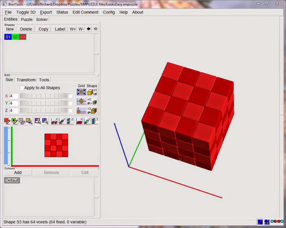
We could simply paint every cell on all four layers but there is a quicker way. Just above the 4x4 grid there is a row of icons. Click the 5th icon to change to Rectangular Selection mode, and also the last icon to toggle "Draw in all Z layers." Now carefully click and drag in the 4x4 grid from top left to bottom right and you should have a large red cube.


Do experiment with these toggle switches when you are ready to learn more about the program. It is also worth checking out the Transform and Tools tabs which hide some very useful functions, like automatically making the internal cubes variable (may or may not be present) when there are internal holes in the puzzle. 'Looks Easy' has 0 internal holes so we don't need that now.

For the final step in this section, let's finish entering the puzzle design. Go to the top and change from Entities to Puzzle.

Click New. Click the red S3 shape, then click the Set Result button.

Click the blue S1 shape, then click +1 four times.

Click the green S2 shape, then click +1 four times.


Now select the Solver tab and click Start to get Burr Tools to show you the solution for this puzzle. Ticking the Disassemble check-box will show you how to solve the puzzle step-by-step by dragging the Move slider.

Note that if the solution involves rotating any of the pieces then Burr Tools will be able to show the final positions but not the disassembly steps.

In part 2 we'll look at how to turn this puzzle into a 3D printable design...

Friday, August 8, 2014

Day 347 - Friday Fail: Self-Intersecting Faces Edition

It seems that the MakerBot Desktop software has an upper bound on the number of "self-intersecting faces" that can be in a model. When I had just a couple of squares hinged together, I didn't have any problems. But with six square faces all with hinges and snaps, there were over 500 of these bad faces (according to MeshLab), caused by triangles that end up somehow sharing parts in the OpenSCAD code. Desktop can't open a file with that much badness, and for a long time I went through a crash/restart/crash/turn-it-off-and-on-again/restart/crash/uninstall/reinstall/forever cycle until I finally figured out that I should maybe go repair the mesh of my file. When I got the number of self-intersecting faces down under 50 by adding additional "fudges" to my OpenSCAD code, MakerBot Desktop could finally open it.

Here's what the remaining 41 self-intersecting faces look like in MeshLab, after selecting Cleaning and Repairing and applying Select Self Intersecting Faces. I could get rid of these also but at this point thing were working so I left well enough alone.


With fudge set to a teeny 0.1, we can sneak in fudges all over the OpenSCAD code with no effect on the printed size of the model, like this:

translate([0-fudge,2*i*snapwidth,0-fudge]) 
cube([height/2+gap+fudge,snapwidth-space+fudge,height+fudge]);

The trick is to make sure that none of your fudges intersect exactly with any of your other fudges. To avoid having two triangles that share the same face you need to keep track of how you've nudged everything - or change the value of fudge - so that you don't fudge-nudge other things into the same place.

Thursday, August 7, 2014

Day 346 - Personalizable Crazy Cube

One really cool thing about a fold-out cube is that you can print things on the faces without using supports and then fold up the cube to get an object with interesting protrusions all over. To print a closed cube with crazy sides would be really unreliable, but to print a flat one is easy. Here's one crazily decorated hinge/snap cube net:


And here is it folded up:


The Customizable Hinge/Snap Cube Net was made in OpenSCAD and then imported into Tinkercad, where we added all the crazy shapes. Here's a public Tinkercad design you can modify to make your own Crazy Cube:


Tinkercad link: https://www.tinkercad.com/things/gu7kcfQV5C3-personalizable-crazy-cube
Thingiverse link: http://www.thingiverse.com/thing:436982

Settings: Printed on a Replicator 2 with .3mm/standard settings, raft but no supports.

Wednesday, August 6, 2014

Day 345 - Customizable hinge/snap Cube net

This week we're attempting to combine three of our previous designs into one:
So far we've managed to get snaps and hinges into the one right-angled model and get everything to fit. Today's code can make corners with two hinges and a snap, or two snaps and one hinge! In other words, we can now make nets for cubes: 


Thingiverse link: http://www.thingiverse.com/thing:436839

Settings: Printed on a MakerBot Replicator 2 at .3mm layer height with standard settings, raft, and no supports. Use the Thingiverse Customizer to set the sizes and clearances however you like.